Investigating pay discrimination in Omega Plc

Omega Group plc- Pay Discrimination
At the last board meeting of Omega Group Plc., the headquarters of a large multinational company, the issue was raised that women were being discriminated in the company, in the sense that the salaries were not the same for male and female executives. A quick analysis of a sample of 50 employees (of which 24 men and 26 women) revealed that the average salary for men was about 8,700 higher than for women. This seemed like a considerable difference, so it was decided that a further analysis of the company salaries was warranted.
The objective is to find out whether there is indeed a significant difference between the salaries of men and women, and whether the difference is due to discrimination or whether it is based on another, possibly valid, determining factor.
Relationship Salary - Gender ?
The data frame omega contains the salaries for the sample of 50 executives in the company.
We calculate summary statistics on salary by gender and also create and print a dataframe where, for each gender, we show the mean, SD, sample size, the t-critical, the SE, the margin of error, and the low/high endpoints of a 95% confidence interval.
# Summary Statistics of salary by gender
mosaic::favstats (salary ~ gender, data=omega) %>%
  knitr::kable(bootstrap_options = c ("striped","hover","condensed","responsive")) %>%
kableExtra::kable_styling()| gender | min | Q1 | median | Q3 | max | mean | sd | n | missing |
|---|---|---|---|---|---|---|---|---|---|
| female | 47033 | 60338 | 64618 | 70033 | 78800 | 64543 | 7567 | 26 | 0 |
| male | 54768 | 68331 | 74675 | 78568 | 84576 | 73239 | 7463 | 24 | 0 |
# Dataframe with two rows (male-female) and having as columns gender, mean, SD, sample size,
# the t-critical value, the standard error, the margin of error,
# and the low/high endpoints of a 95% condifence interval

gender_stats <- omega %>%
  group_by(gender) %>%
  summarise(mean_salary=mean(salary),
            sd_salary=sd(salary),
            count=n(),
            t_critical=qt(0.975,count-1),
            se=sd_salary/sqrt(count),
            margin_of_error=t_critical*se,
            lower_ci=mean_salary-margin_of_error,
            upper_ci=mean_salary+margin_of_error)

gender_stats %>%
  knitr::kable(bootstrap_options = c ("striped","hover","condensed","responsive")) %>%
kableExtra::kable_styling()| gender | mean_salary | sd_salary | count | t_critical | se | margin_of_error | lower_ci | upper_ci |
|---|---|---|---|---|---|---|---|---|
| female | 64543 | 7567 | 26 | 2.06 | 1484 | 3056 | 61486 | 67599 |
| male | 73239 | 7463 | 24 | 2.07 | 1523 | 3151 | 70088 | 76390 |
Looking at the summary statistics above, we can conclude that the mean salary of male employees is larger than the female salary with the means being 73200 $ (3 sf) and 64500 $ (3sf) respectively. The medians and quartiles show a similar relationship, ie males having higher earnings than females. Calculating 95% confidence intervals for the two genders we can observe that these two do not overlap and thus we conclude that indeed the mean salary between males and females is significantly different, with males earning more.
We also run a hypothesis test, assuming as a null hypothesis that the mean difference in salaries is zero, or that, on average, men and women make the same amount of money.
\(H_0: \mu_{male}-\mu_{female}= 0\) vs \(H_1: \mu_{male}-\mu_{female}\neq 0\)
# hypothesis testing using t.test()
t.test(salary~gender,data=omega)
##
## Welch Two Sample t-test
##
## data: salary by gender
## t = -4, df = 48, p-value = 2e-04
## alternative hypothesis: true difference in means between group female and group male is not equal to 0
## 95 percent confidence interval:
## -12973 -4420
## sample estimates:
## mean in group female mean in group male
## 64543 73239# hypothesis testing using infer package
hyp_by_gender <- omega %>%
# specify variables
specify(salary~gender) %>%
# assume independence, i.e, there is no difference
hypothesize(null = "independence") %>%
# generate 1000 reps, of type "permute"
generate(reps = 1000, type = "permute") %>%
# calculate statistic of difference, namely "diff in means"
calculate(stat = "diff in means", order = c("male", "female"))
mean_difference<- omega %>%
specify(salary~gender) %>%
calculate(stat="diff in means",
order=c("male","female"))
hyp_by_gender %>%
get_p_value(obs_stat = mean_difference , direction = "two_sided") %>%
knitr::kable(bootstrap_options = c ("striped","hover","condensed","responsive")) %>%
kableExtra::kable_styling()| p_value |
|---|
| 0 |
The hypothesis tests, both using the t test and the bootstrap simulation, confirm our previous observation. The p-value is approximately 0 and hence the null hypothesis is rejected and we conclude that the means are significantly different. There is a difference between average male and female earnings.
Relationship Experience - Gender?
At the board meeting, someone raised the issue that there was indeed a substantial difference between male and female salaries, but that this was attributable to other reasons such as differences in experience. A questionnaire send out to the 50 executives in the sample reveals that the average experience of the men is approximately 21 years, whereas the women only have about 7 years experience on average (see table below).
# Summary Statistics of salary by gender
favstats (experience ~ gender, data=omega) %>%
  knitr::kable(bootstrap_options = c ("striped","hover","condensed","responsive")) %>%
kableExtra::kable_styling()| gender | min | Q1 | median | Q3 | max | mean | sd | n | missing |
|---|---|---|---|---|---|---|---|---|---|
| female | 0 | 0.25 | 3.0 | 14.0 | 29 | 7.38 | 8.51 | 26 | 0 |
| male | 1 | 15.75 | 19.5 | 31.2 | 44 | 21.12 | 10.92 | 24 | 0 |
We will calculate CIs and see if they overlap:
experience_stats <- omega %>%
  group_by(gender) %>%
  summarise(mean_experience=mean(experience),
            sd_experience=sd(experience),
            count=n(),
            t_critical=qt(0.975,count-1),
            se=sd_experience/sqrt(count),
            margin_of_error=t_critical*se,
            lower_ci=mean_experience-margin_of_error,
            upper_ci=mean_experience+margin_of_error)

experience_stats %>%
  knitr::kable(bootstrap_options = c ("striped","hover","condensed","responsive")) %>%
kableExtra::kable_styling()| gender | mean_experience | sd_experience | count | t_critical | se | margin_of_error | lower_ci | upper_ci |
|---|---|---|---|---|---|---|---|---|
| female | 7.38 | 8.51 | 26 | 2.06 | 1.67 | 3.44 | 3.95 | 10.8 |
| male | 21.12 | 10.92 | 24 | 2.07 | 2.23 | 4.61 | 16.52 | 25.7 |
The 95% confidence intervals do not overlap. The confidence interval for male experience looks to be significantly higher than female. We can conclude that there is a significant difference of average experience across genders.
We perform similar analyses as in the previous section.
\(H_0: \mu_{male}-\mu_{female}= 0\) vs \(H_1: \mu_{male}-\mu_{female}\neq 0\)
t.test(experience~gender,data=omega)##
## Welch Two Sample t-test
##
## data: experience by gender
## t = -5, df = 43, p-value = 1e-05
## alternative hypothesis: true difference in means between group female and group male is not equal to 0
## 95 percent confidence interval:
## -19.35 -8.13
## sample estimates:
## mean in group female mean in group male
## 7.38 21.12The hypothesis test confirms our previous findings. The p-value is approximately 0 so we reject the null hypothesis and conclude that average experience of males and females is significantly different. This conclusion can be used as the reason why males earn more than females in the company which is what we discovered in our previous analysis.
Relationship Salary - Experience ?
Someone at the meeting argues that clearly, a more thorough analysis of the relationship between salary and experience is required before any conclusion can be drawn about whether there is any gender-based salary discrimination in the company.
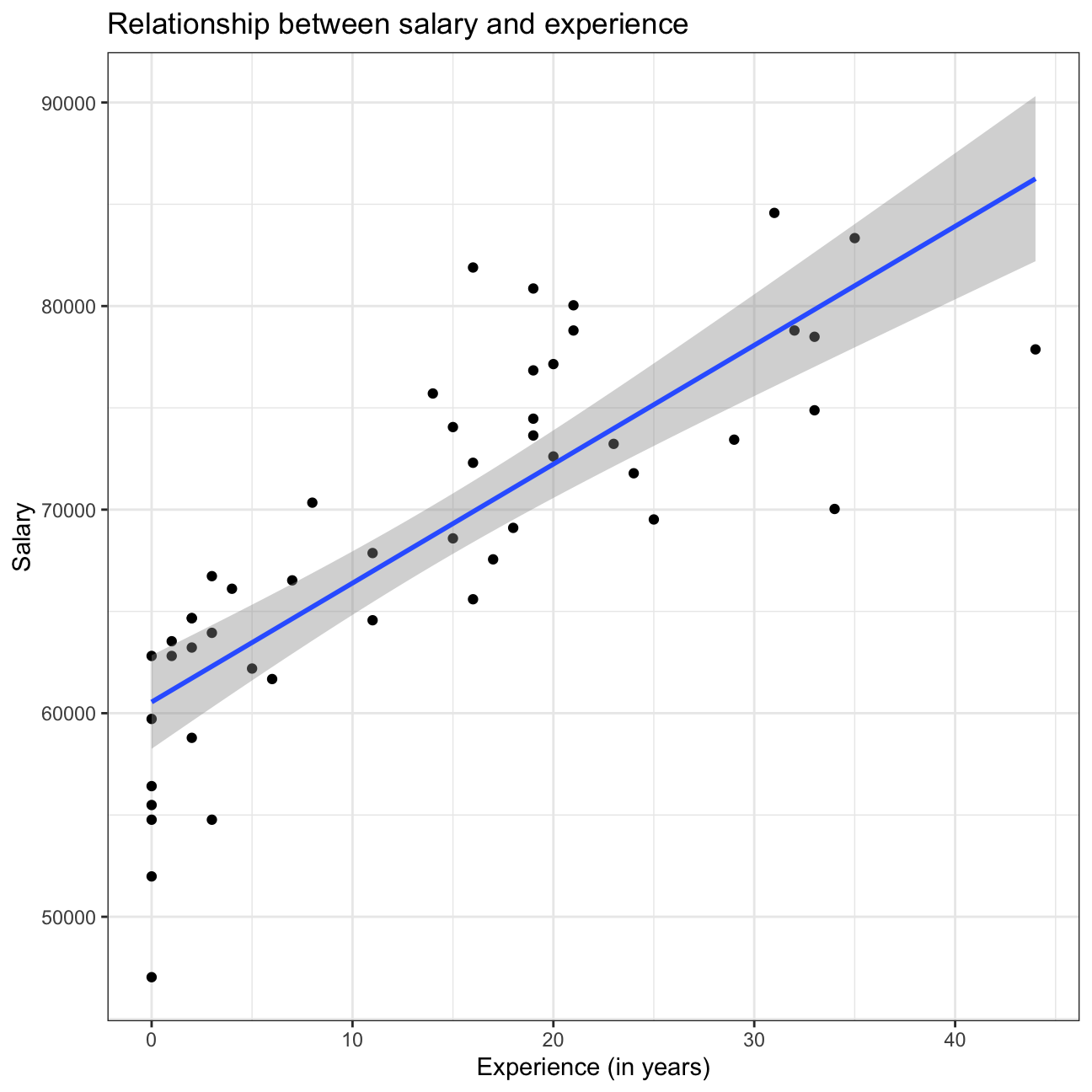
Let’s analyse the relationship between salary and experience and draw a scatterplot to visually inspect the data.
ggplot(omega, aes(x=experience, y=salary))+
  geom_point()+
  theme_bw()+
  geom_smooth(method=lm)+
  labs(
    title="Relationship between salary and experience",
    x="Experience (in years)",
    y="Salary"
  )
Check correlations between the data
We use GGally:ggpairs() to create a scatterplot and correlation
matrix.
omega %>%
  select(gender, experience, salary) %>% #order variables they will appear in ggpairs()
  ggpairs(aes(colour=gender, alpha = 0.3))+
  theme_bw()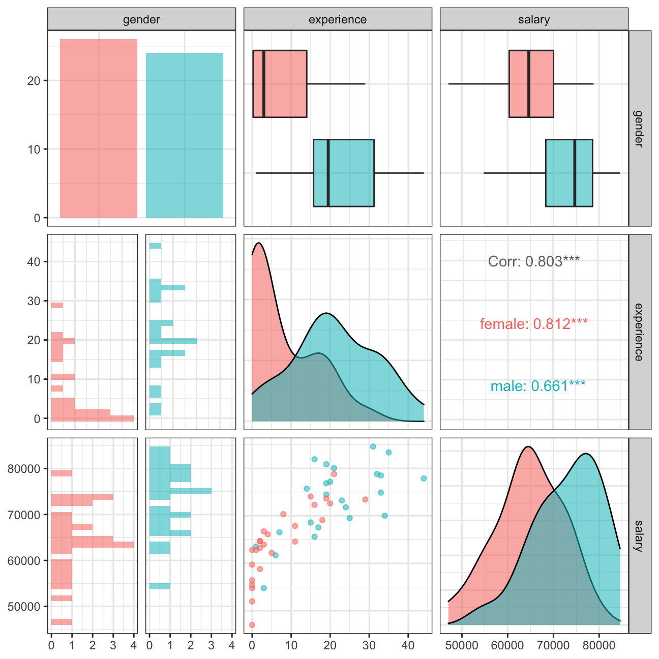
From the scatterplot, it is evident that as years of experience increase the salary increases as well. There is a positive correlation between the two variables. This is expected as normally more experienced individual are at higher, managerial positions which are paid more.
This increase in pay is more evident for the first 20 years of experience and after that it looks like it levels off. This is also because there aren’t many employees with experience more than 25 years, and those must be at the highest earning potential in the company.
Now, looking at the gender as well, we earlier concluded that males have more experience than females and as salary increases with experience, it is reasonable that males earn more than females.
that the US has been experiencing a slight increase in the percentage of GDP in household spending of about 5% and has a trade deficit over the years that is as low as 5%. Whereas for Germany where Household spending seems to slightly decrease, net exports have increased from having a trade deficit a few decades ago to a surplus of about 8%.
Generally, for developed countries in the long term, the proportions of all four components of GDP should see less variability than the proportions for emerging countries. This is exactly what is shown by the comparison between developed countries (Germany, US) and emerging economy (India).