General Social Survey (GSS)

The General Social Survey (GSS) gathers data on American society in order to monitor and explain trends in attitudes, behaviors, and attributes. Many trends have been tracked for decades, so one can see the evolution of attitudes, etc in American Society.
In this assignment I analyzed data from the 2016 GSS sample data, using it to estimate values of population parameters of interest about US adults. The GSS sample data file has 2867 observations of 935 variables, but only a few of these variables are of interest.
I started by creating 95% confidence intervals for population parameters. The variables we have are the following:
- hours and minutes spent on email weekly. The responses to these questions are recorded in the
emailhrandemailminvariables. For example, if the response is 2.50 hours, this would be recorded as emailhr = 2 and emailmin = 30. snapchat,instagrm,twitter: whether respondents used these social media in 2016sex: Female - Maledegree: highest education level attained
Instagram and Snapchat, by sex
These are the relevant steps to calculate the population proportion of Snapchat or Instagram users in 2016:
- Create a new variable,
snap_instathat is Yes if the respondent reported using any of Snapchat (snapchat) or Instagram (instagrm), and No if not. For reported NA values, the value in the new created variable is also NA.
#Creating a new variable 'Snap_Intsa'
snap_insta <- gss %>%
  mutate(snap_insta = if_else(snapchat == "NA" & instagrm == "NA", "NA",
if_else(snapchat=="Yes" | instagrm == "Yes", "Yes", "No")))- Calculate the proportion of Yes’s for
snap_instaamong those who answered the question, i.e. excluding NAs.
#Calculating proportion of 'snap_insta' users
snap_insta %>%
  filter(snap_insta != "NA") %>%
  summarize(
    Proportion_Insta_Snap = count(snap_insta=="Yes") / n())
## # A tibble: 1 × 1
## Proportion_Insta_Snap
## <dbl>
## 1 0.375- Using the CI formula for proportions and thus constructing 95% CIs for men and women who used either Snapchat or Instagram
# CI for Male population
male_proportion <- snap_insta %>%
  filter(sex == "Male", snap_insta != "NA") %>%
  summarize(
    proportion = count(snap_insta == "Yes")/n(),
    se = sqrt((proportion*(1 - proportion)/n())),
    lower_ci = proportion - 1.96*se, #we are using normal distribution to approximate
                                     #binomial distribution and directly use 1.96 as the critical value
    upper_ci = proportion + 1.96*se) %>%
  knitr::kable(caption = "95% CI for men who used either Snapchat or Instagram") %>%
  kableExtra::kable_styling()

# CI for Female population
female_proportion <- snap_insta %>%
  filter(sex == "Female", snap_insta != "NA") %>%
  summarize(
    proportion = count(snap_insta == "Yes")/n(),
    se = sqrt((proportion*(1 - proportion)/n())),
    lower_ci = proportion - 1.96*se,
    upper_ci = proportion + 1.96*se) %>%
  knitr::kable(caption = "95% CI for women who used either Snapchat or Instagram") %>%
  kableExtra::kable_styling()

#print out CIs
male_proportion| proportion | se | lower_ci | upper_ci |
|---|---|---|---|
| 0.318 | 0.019 | 0.281 | 0.356 |
female_proportion| proportion | se | lower_ci | upper_ci |
|---|---|---|---|
| 0.419 | 0.018 | 0.384 | 0.454 |
As we observe the two confidence intervals do not overlap. This means that there is indeed a significant difference in the proportion of women using Snapchat or Instagram compared to men. A larger proportion of women tend to use these socials.
Twitter, by education level
Next, the population proportion of Twitter users by education level in 2016 is estimated:
There are 5 education levels in variable degree which, in ascending order of years of education, are Lt high school, High School, Junior college, Bachelor, Graduate.
- A new variable
bachelor_graduateis constructed that is Yes if the respondent has either aBachelororGraduatedegree. I then calculated the proportion ofbachelor_graduatewho do (Yes) and who don’t (No) use twitter.
#tidy data and count
twitter_bachelor <- gss_degree %>%
  filter(bachelor_graduate == "Yes", twitter != "NA") %>%
  group_by(bachelor_graduate, twitter) %>%
  count()

#calculate proportions
twitter_bachelor_proportions <- twitter_bachelor %>%
  pivot_wider(names_from = twitter, values_from = n) %>%
  summarize(
    Bachelors_using_twitter = Yes/sum(Yes,No),
    Bachelors_not_using_twitter = 1 - Bachelors_using_twitter
  ) %>%
  select(c("Bachelors_using_twitter", "Bachelors_not_using_twitter")) %>%
  knitr::kable(caption = "Proportions for bachelor graduates using and not using Twitter") %>%
  kableExtra::kable_styling()

twitter_bachelor_proportions| Bachelors_using_twitter | Bachelors_not_using_twitter |
|---|---|
| 0.233 | 0.767 |
- Using the CI formula for proportions I constructed two 95% CIs for
bachelor_graduatevs whether they use (Yes) and don’t (No) use twitter.
#construct CI using formula
twitter_bachelor_95 <- twitter_bachelor %>%
  mutate(
    count = sum(twitter_bachelor$n),
    proportion = n/count,
    se_twitter = sqrt((proportion * (1-proportion))/count),
    lower_ci =  proportion - 1.96*se_twitter,
    upper_ci= proportion + 1.96*se_twitter) %>%
  select(c("bachelor_graduate","twitter", "lower_ci", "upper_ci")) %>%
  knitr::kable(caption = "95% CIs for bachelor graduates who use and do not use Twitter") %>%
  kableExtra::kable_styling()

twitter_bachelor_95| bachelor_graduate | lower_ci | upper_ci | |
|---|---|---|---|
| Yes | No | 0.729 | 0.804 |
| Yes | Yes | 0.196 | 0.271 |
These two confidence intervals do not overlap. There is a significant difference in the proportion of bachelor graduates who do and who do not use Twitter. Therefore, we can make inferences about twitter usage according to whether people are bachelor graduates or not.
Email usage
Let’s estimate the population parameter on time spent on email weekly:
- Create a new variable called
emailthat combinesemailhrandemailminto reports the number of minutes the respondents spend on email weekly.
#Creating a new variable
email_time <- gss %>%
  mutate(
    email = as.numeric(emailhr) * 60 + as.numeric(emailmin))

email_time
## # A tibble: 2,867 × 8
## emailmin emailhr snapchat instagrm twitter sex degree email
## <chr> <chr> <chr> <chr> <chr> <chr> <chr> <dbl>
## 1 0 12 NA NA NA Male Bachelor 720
## 2 30 0 No No No Male High school 30
## 3 NA NA No No No Male Bachelor NA
## 4 10 0 NA NA NA Female High school 10
## 5 NA NA Yes Yes No Female Graduate NA
## 6 0 2 No Yes No Female Junior college 120
## 7 0 40 NA NA NA Male High school 2400
## 8 NA NA Yes Yes No Female High school NA
## 9 0 0 NA NA NA Male High school 0
## 10 NA NA No No No Male Junior college NA
## # … with 2,857 more rows- A visualisation of the distribution is seen below followed by summary statistics of the mean and the median number of minutes respondents spend on email weekly.
#Visualizing the new variable 'Email'
ggplot(email_time,
       aes(x= email))+
  geom_density()+
  theme_bw() +
  labs (
    title = "Time Spent on email",
x = "Minutes spent on email weekly") 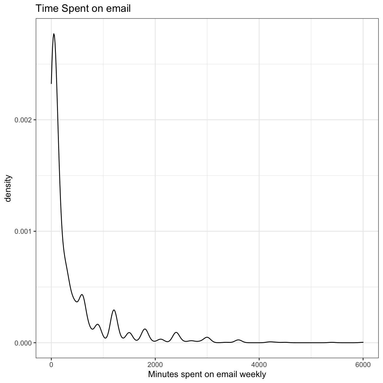
#calculate mean and median
email_time %>%
  summarise(mean_email_time = mean(email, na.rm=TRUE),
            median_email_time = median(email, na.rm=TRUE))
## # A tibble: 1 × 2
## mean_email_time median_email_time
## <dbl> <dbl>
## 1 417. 120The median is a better measure since the density of time spent is significantly right skewed and extreme values in the right tail pull the mean away from the center. This skewness implies extreme outliers that don’t reflect the typical American’s email usage.
The median is less affected by such extreme values.
- Using the
inferpackage, I calculated a 95% bootstrap confidence interval for the mean amount of time Americans spend on email weekly.
#construct CI using bootstrap
set.seed(1998)
library(infer)

bootstrap_email <- email_time %>%
  specify(response = email) %>%
  generate(reps = 1000, type = "bootstrap") %>%
  calculate(stat = "mean")

bootstrap_ci <- bootstrap_email %>%
  get_ci(level = 0.95, type = "percentile") %>%
  #"humanize" time units to [__ hrs __ mins]
  mutate(lower_ci = paste(paste(385 %/% 60, "hrs"),
                          paste(385 %% 60, "mins")),
         upper_ci = paste(paste(448 %/% 60, "hrs"),
                          paste(448 %% 60, "mins"))) %>%
  knitr::kable(caption = "95% CI for weekly email usage of Americans") %>%
  kableExtra::kable_styling()
bootstrap_ci| lower_ci | upper_ci |
|---|---|
| 6 hrs 25 mins | 7 hrs 28 mins |
Since we are calculating weekly email, roughly 7 hours per week or 1 hour per day seems normal.